Analyse failures by failure mode (competing risks)
Before you start: Life data with a column naming each failure's mode (blank for a unit still running).
Most equipment can fail in more than one way. A pump can wear out its bearings, leak at the seal or break its impeller. Lumping every failure into one distribution hides which mode drives the losses, and when. The modes also compete: a pump that fails from a seal leak at 2,000 hours never gets the chance to wear out its bearings at 4,000.
A competing-risks fit handles that properly. For each mode, it gives the cumulative incidence: the share of units that fail from that mode by each time, while the other modes are still acting. The modes add up to the chance of failing from any cause.
Your data
One row per unit: its time, and the mode it failed from. Leave the mode blank for a unit that is still running.
pump,hours,failure_mode,site
P-01,4810,bearing wear,A
P-03,920,impeller damage,A
P-05,4720,,A
P-08,1960,seal leak,B
The sample Pump failures by mode has 72 pumps like this: 50 failed from three modes and 22 still running.
Fit by failure mode
Go to Modelling → Life models, start a new model and choose Fit to data. Pick your file or dataset. In the Data step, choose the mode column as Failure mode (optional). The step reminds you that a blank mode is a unit still running.
You can still map Failed or still running? if your file has a status column as well. Otherwise the blank modes say which units are running.
Press Next. The Model step now reads Failure modes from "failure_mode" — they are fitted as competing risks, and offers Competing risks (by failure mode). No distribution is assumed: the curves come straight from the data.
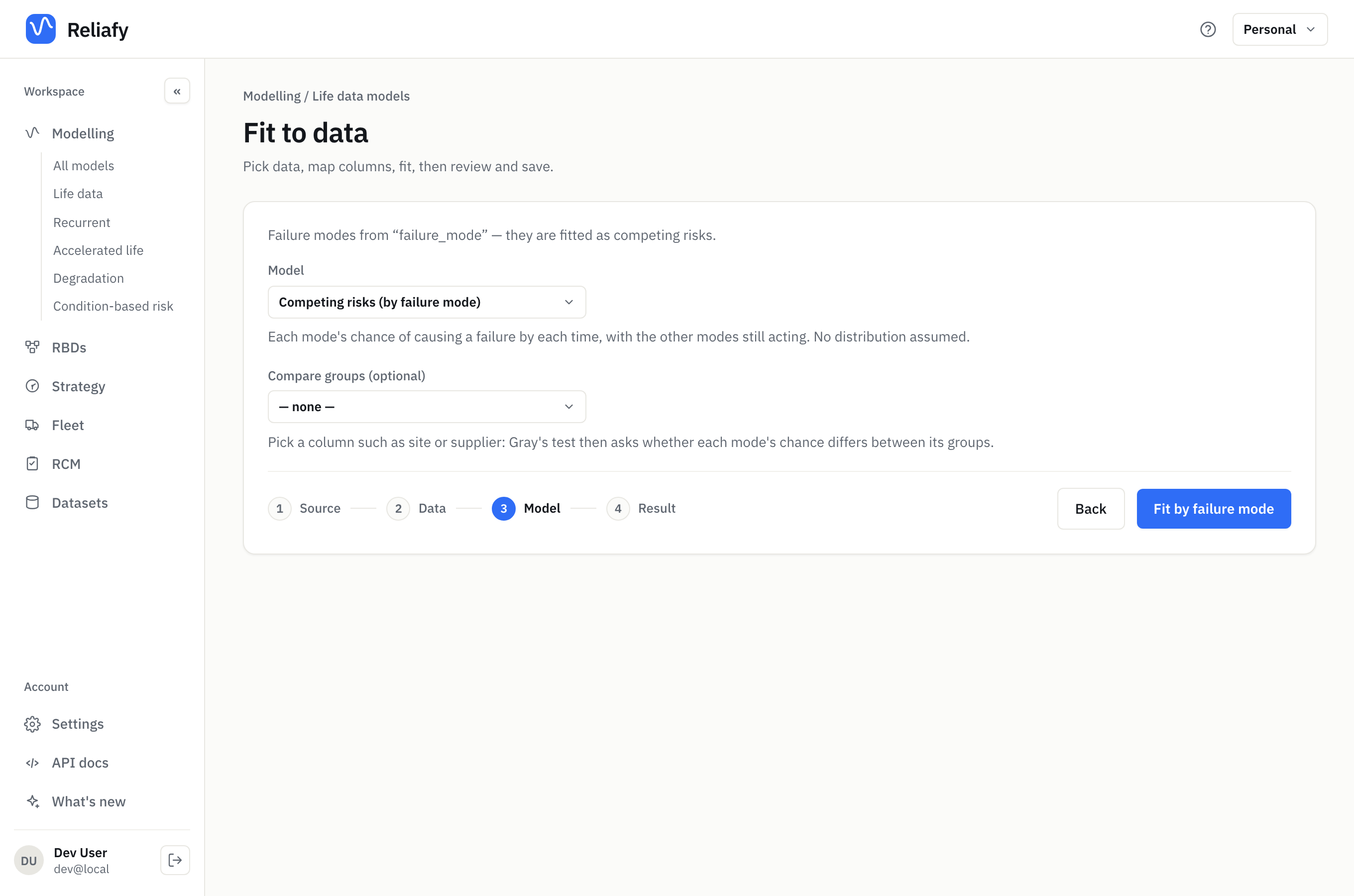
Compare groups (optional) takes a column such as site or supplier. Leave it blank for now. Press Fit by failure mode, then Save model.
Read the result
The Cumulative incidence chart stacks the modes. Each band is one mode's share; the top edge is the chance of failing from any mode, with its 95% band in grey. Switch Show to Each mode to see each mode on its own, with its own band.
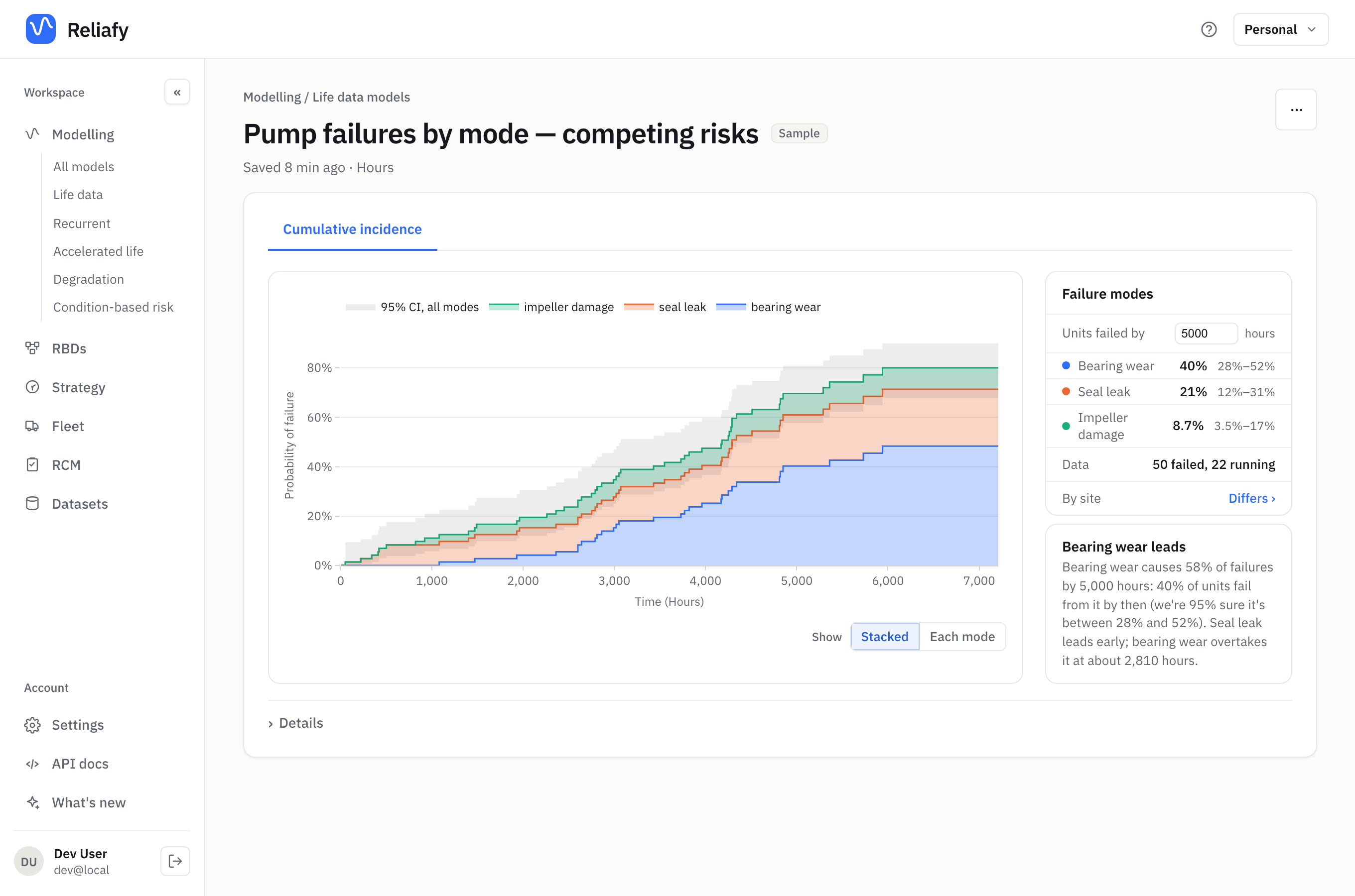
The Failure modes panel reads the curves at one time. Type any time into Units failed by. For the sample at 5,000 hours:
| Mode | Units failed from it by 5,000 hours | 95% interval |
|---|---|---|
| Bearing wear | 40% | 28%–52% |
| Seal leak | 21% | 12%–31% |
| Impeller damage | 8.7% | 3.5%–17% |
The reading under it says it in words: Bearing wear causes 58% of failures by 5,000 hours … Seal leak leads early; bearing wear overtakes it at about 2,810 hours. That's the practical point. Early in life, seal leaks are the problem to fix. Later, bearing wear takes over, and that's what a replacement interval should target.
Why not fit each mode separately?
A common shortcut fits a distribution to one mode and treats every other failure as "still running". That answers a different question: how long a unit would last if no other mode existed. Add those up and you over-count, because a unit can only fail once. Cumulative incidence counts each unit once, by the mode that actually ended its life.
Do the modes differ between groups?
Fit again with a column in Compare groups (optional), such as site. The
panel gains a By site row; click it for Gray's test on each mode. The
sample model already has this:
Seal leak differs by site (Gray's test, p < 0.001): by 5,000 hours, 35% of site B's units fail from it, against 6.2% of site A's.
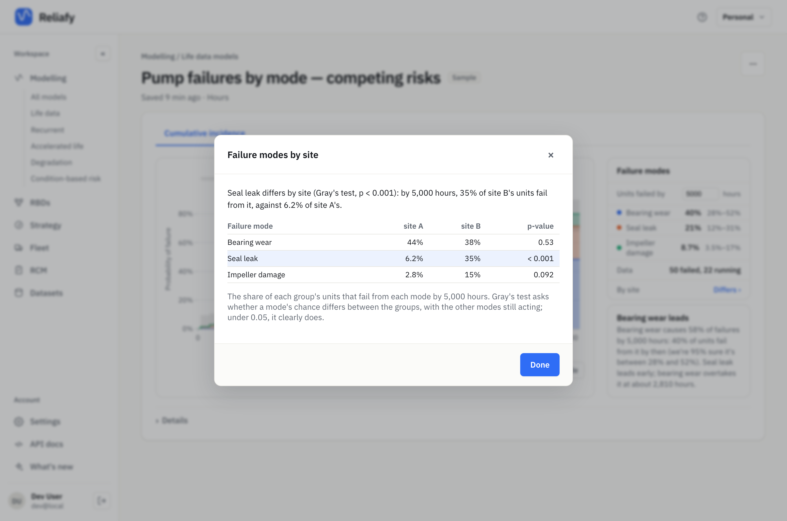
Bearing wear (p = 0.53) and impeller damage (p = 0.092) don't clearly differ. So the extra failures at site B are seal leaks: look at what is different about how site B installs or runs its seals.
What drives each mode
To measure how a factor changes each mode, tick it as a covariate in the Data step, under Advanced (regression): covariates. The Model step then offers two regressions by mode:
- Cause-specific Cox: how each covariate changes the failure rate from each mode, among units still running. Use it to understand why a mode happens.
- Fine-Gray: how each covariate changes the chance of failing from each mode with the other modes acting. Use it to predict how many units a mode will take.
The result gains a Coefficients tab. With duty_pct as the covariate, the
sample gives:
Each +1 in duty_pct multiplies the bearing wear failure rate by 1.14.
| Failure mode | Hazard ratio | 95% interval | p-value |
|---|---|---|---|
| Bearing wear | 1.14 | 1.08–1.21 | < 0.001 |
| Impeller damage | 1 | 0.939–1.07 | 0.9 |
| Seal leak | 0.973 | 0.932–1.02 | 0.22 |
A ratio above 1 makes the mode come sooner; below 1, later. Here duty drives bearing wear only: each extra 10% of duty multiplies the bearing wear rate by about 1.14¹⁰ ≈ 3.7, while seals and impellers don't care.
Where to go next
- To compare groups without splitting by mode, or to plan a trial of a fix, see find out whether a change made a difference.
- To fit a single distribution to all failures together, see fit your first life model.
- For covariates without failure modes, see fit a model with covariates.
The cumulative incidence (Aalen–Johansen, with Aalen's 95% bounds) and Gray's test come from SurPyval, an open-source Python library.