Fit a model with covariates (regression)
Before you start: Life data with one or more columns that might affect life: a temperature, a load, a duty, a site. For a load that changes during a unit's life, one row per stretch at each value.
A plain life model gives one answer for every unit. Real units don't all run the same way. Seals on a hot line fail sooner than seals on a cool one, and a pump at 90% duty wears faster than one at 60%. A regression model, also called a covariate model, measures how much each of those factors changes life. You can then ask the model about any operating condition, including ones you haven't tested.
The factors are called covariates. Use one when you want to know how much it matters. If you only want to know whether two groups differ, comparing them is simpler: see find out whether a change made a difference.
Your data
One row per unit, with its time, whether it failed, and a column per covariate:
hours,censored,temp_C,load
1350,0,60,0.5
2200,1,60,0.5
950,0,60,0.9
The sample Valve seal life vs. temperature & load is 32 seals like this, tested at 60, 80 and 100 °C and at two loads.
Add the covariates
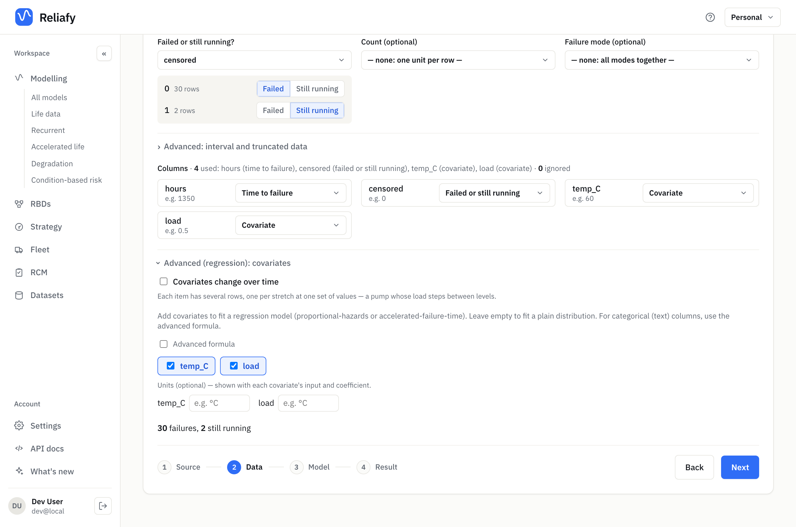
Start a new model under Modelling → Life models and choose Fit to data. Map the time and status columns in the Data step as usual (see fit your first life model). Then open Advanced (regression): covariates and tick each covariate column. Give each one a unit if you like (°C, kN); it's shown with its input and its coefficient.
Text columns, such as a site or a supplier, need Advanced formula. Write a
formula over your columns, such as temp_C + load + site, and categories are
expanded for you. A formula can also hold interactions (temp_C:load) when
one factor's effect depends on another.
Choose a regression
With covariates ticked, the Model step offers regressions instead of plain distributions, in four families. They differ in how a covariate acts:
- Proportional hazards (PH): a covariate multiplies the failure rate. Each +1 °C makes failure, say, 15% more likely at every age. This is the usual starting point. Cox PH (semi-parametric) does the same without assuming a distribution for the baseline.
- Accelerated failure time (AFT): a covariate speeds up or slows down time. Each +1 °C makes the seal age as if 2.5% more hours had passed. This is the natural reading for a stress that wears a part out faster.
- Proportional odds (PO): a covariate multiplies the odds of having failed. Its effect fades with age.
- Additive hazards (AH): a covariate adds a fixed amount to the failure rate rather than multiplying it.
Under More models there are semi-parametric versions (Lin-Ying additive hazards, proportional odds, Buckley-James AFT) and shared frailty models. A frailty model is for units grouped by site or batch that share a hidden risk: choose its Group by (site or batch) column and the fit says how much the groups differ.
For Cox PH, Advanced Cox options set how Tied failure times are handled (Efron by default), a column to Stratify by (each level gets its own baseline, with shared covariate effects), and a column to Cluster robust errors by when several rows come from one unit.
For a stress you want to extrapolate to use conditions, an accelerated life model is the purpose-built tool. Choose a regression here when the covariates describe how units are run in service.
Read the effects
Fit the seal data with Weibull PH (the sample model Valve seal life — Weibull PH on temp & load is this fit) and open the Coefficients tab:
| Covariate | β | 95% interval | Hazard ratio e^β |
|---|---|---|---|
| temp_C | 0.138 | 0.093 to 0.183 | 1.148 |
| load | 5.32 | 3.02 to 7.63 | 205 |
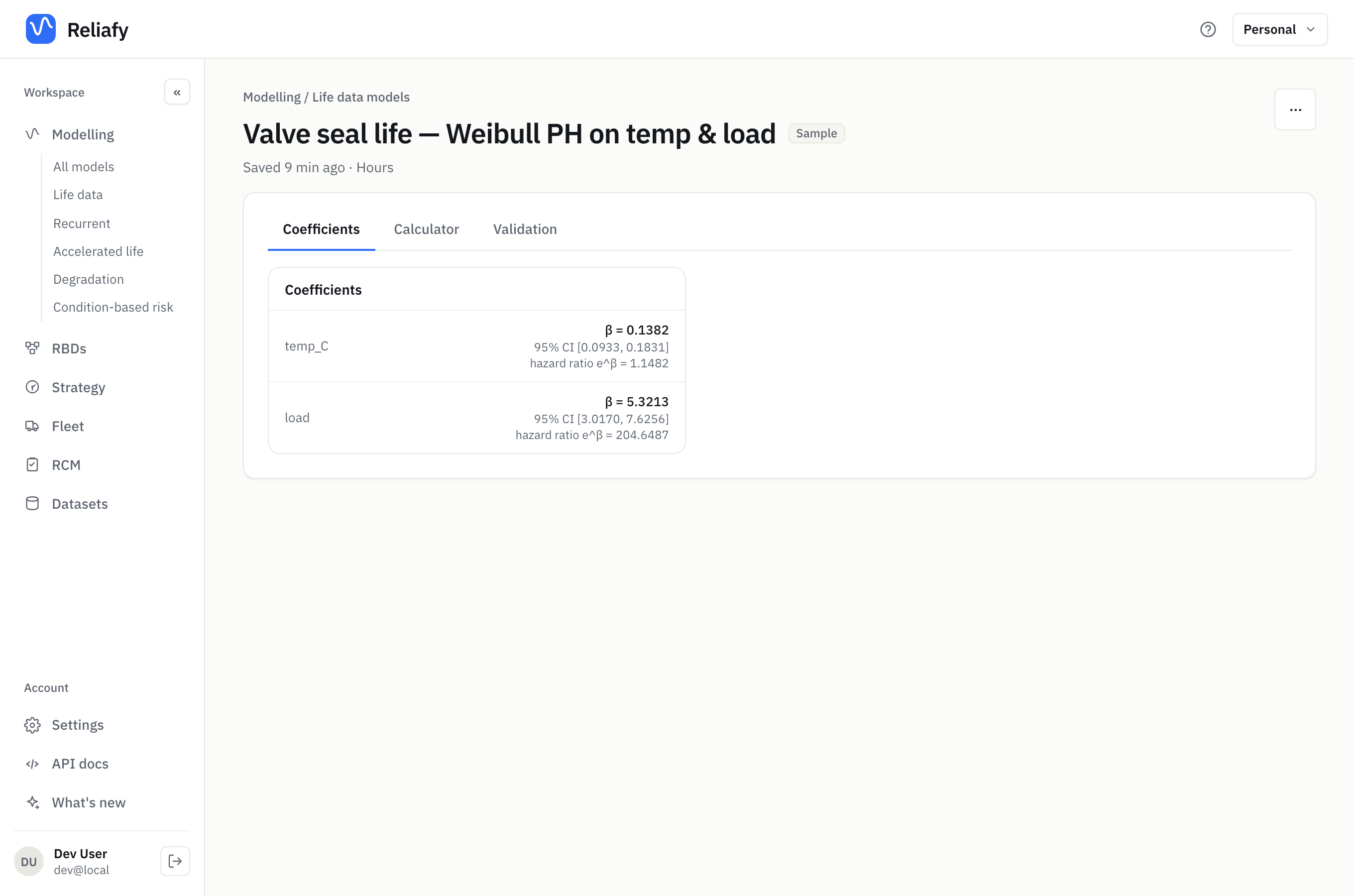
Read the hazard ratio as "per +1 of the covariate, the failure rate is multiplied by this". So each extra degree multiplies it by 1.148, and 10 °C hotter multiplies it by 1.148¹⁰ ≈ 4. The load's ratio looks huge only because load runs from 0.5 to 0.9: going from 0.5 to 0.9 multiplies the failure rate by e^(5.32 × 0.4) ≈ 8.4.
An interval for β that doesn't include 0 (a ratio that doesn't include 1) means the covariate clearly matters. Both do here.
An AFT model reports a time ratio instead. For the same data, Weibull AFT gives temp_C a time ratio of 1.025: each extra degree makes the seal age 2.5% faster. The two views agree. For a Weibull, the hazard ratio is the time ratio raised to the shape β: 1.025^5.58 ≈ 1.148.
Ask about one operating condition
The Calculator tab answers for the covariate values you type under Covariates: reliability at a time, a time at a reliability, the B-lives and the MTTF, each with its bound. + Add combination draws another set of values on the same chart, such as the same seal at 60 °C and at 100 °C.
Check the model holds
The Validation tab asks two questions.
How good is this model? Harrell's C is how often the model ranks the unit that failed first as the riskier one (0.87 for the seals: strong). The integrated Brier score is the prediction error, against one survival curve for every unit. Here the covariates cut it by 63%.
Does the model hold? For PH models, the Grambsch-Therneau test checks the core assumption: that each covariate's effect stays the same over time. A p-value above 0.05 (0.69 here) means one hazard ratio per covariate describes the data. Test details and residuals opens the per-covariate tests and the Schoenfeld, martingale and deviance residual plots. If the assumption fails, try an AFT or PO model, or stratify a Cox model on the offending column.
Covariates that change over time
Sometimes a covariate changes during a unit's life. A pump runs at 60% load for 1,500 hours, then 90% until it fails. Give each unit one row per stretch at one set of values:
pump,start_h,stop_h,censored,load_pct
P-01,0,1500,1,90
P-01,1500,3700,1,75
P-01,3700,4289,0,90
Under Advanced (regression): covariates, tick Covariates change over time and choose how the rows are laid out:
- Start and stop rows: each row is one stretch, from Start of the row to End of the row, and Did the row end in a failure? says whether the unit failed at its end.
- Timeline rows: each row is a change, with its values holding until the unit's next row. The last row is the failure or removal.
Then choose the Item column that says which unit each row belongs to. Reliafy recognises start and stop columns and turns this on for you when it can. The Model step then offers the regressions that can follow a changing covariate (the PH, AFT, PO and AH families and Cox PH).
The result's Calculator takes a Covariate schedule: the value from time 0, then + Add a change for each step. The sample Pump bearings — Weibull PH on changing load opens on 60% load, stepping to 90% at 4,800 hours. The curve bends down at the step, and the answer is for that schedule: R(6,000 hours) = 36%, at least 26% at 90% confidence.
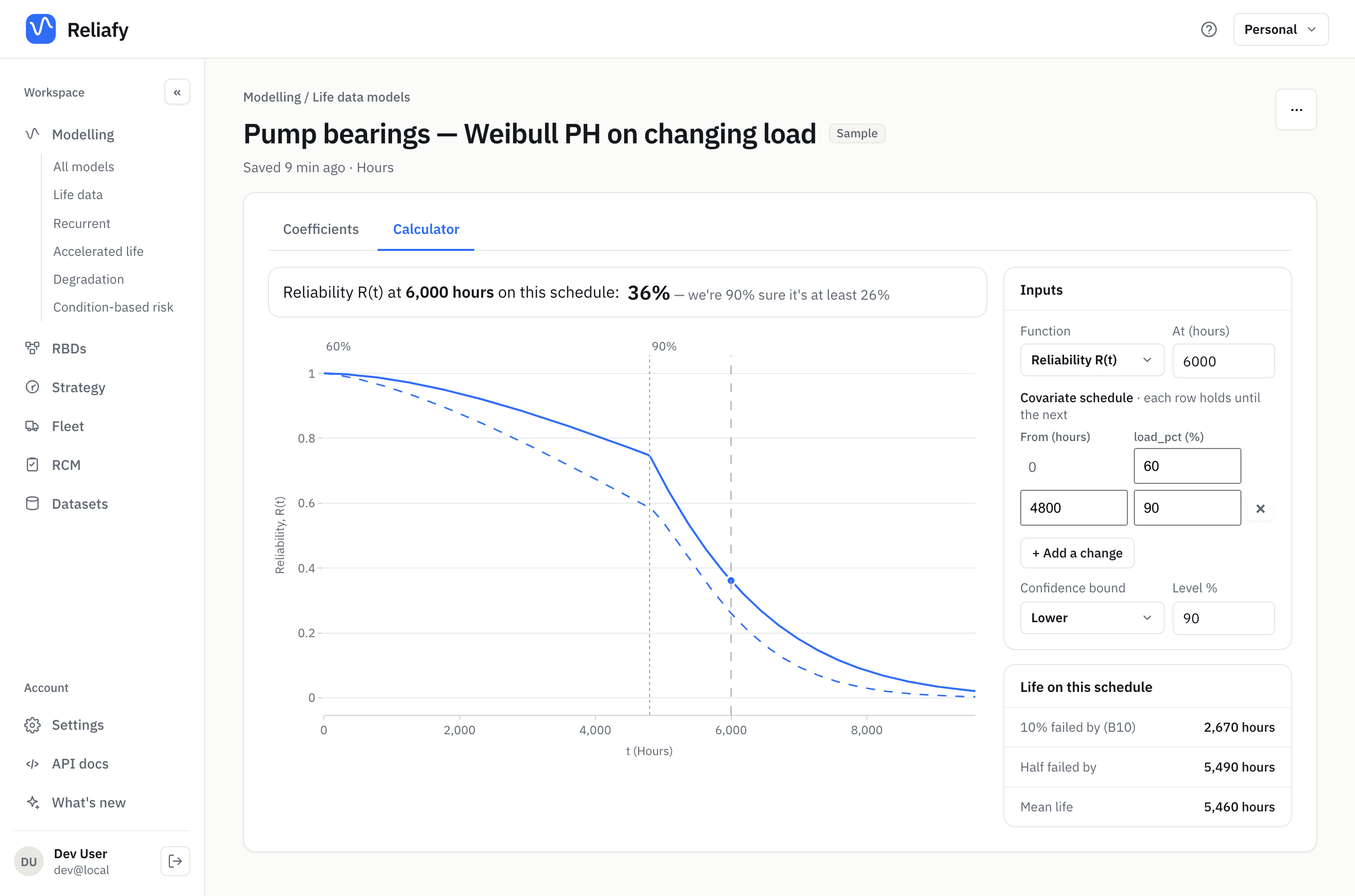
Its Coefficients tab says it in words: every +10% in load_pct multiplies the hazard by 1.74 (95% interval 1.19 to 2.55).
Use it elsewhere
Save the model and it can drive a block in a reliability block diagram. The block takes the covariate values to run at. In a non-repairable diagram it can take a schedule of them over the mission instead.
Where to go next
- For failure modes as well as covariates, see competing risks: Cause-specific Cox and Fine-Gray give the effects mode by mode.
- To predict life at a use stress from a high-stress test, see accelerated life testing.
- For a condition reading that drifts with age (vibration, wear, oil), see rank running units by risk.
The regressions come from SurPyval, an open-source Python library.